Modeling spatially varying gene correlation across 2D space

library(spCorr)
library(ggplot2)
library(dplyr)
library(tidyr)
library(viridis)

Introduction

This tutorial demonstrates how to use spCorr to (i) infer spot-level gene–gene correlations for specified gene pairs, and (ii) identify gene pairs exhibiting spatially varying correlation (SVC) patterns across a 2D spatial space.

Prepare input data

In this example, we analyze a subset of the human oral squamous cell carcinoma (OSCC) dataset generated using the 10x Visium platform (sample 2 from Arora et al., 2023). We focus on transcription factor (TF)–target gene pairs curated from the TRRUST v2 database.

## Load example spatial transcriptomics data
# It contains two objects: counts (gene expression matrix) and cov_mat (spot-level covariates)
load(url("https://figshare.com/ndownloader/files/58905268"))
# counts: gene expression count matrix (genes x spots)
print(dim(counts))
#> [1] 15624  1747

# cov_mat: spot spatial coordinates and other spot-level covariates
print(dim(cov_mat))
#> [1] 1747    5
head(cov_mat)
#>                       x1    x2 cluster_annotations         pathologist_anno.x
#> AAACATTTCCCGGATT-2 17022 16020                core                        SCC
#> AAACCGGGTAGGTACC-2 12218  6043                  nc Lymphocyte Negative Stroma
#> AAACCGTTCGTCCAGG-2 14740  8064                edge                        SCC
#> AAACCTAAGCAGCCGG-2 18025 13992                  nc                        SCC
#> AAACGAGACGGTTGAT-2 10469 13427                edge                        SCC
#> AAACGGGCGTACGGGT-2 18027 15149          transitory                        SCC
#>                    tumor_annotations
#> AAACATTTCCCGGATT-2             tumor
#> AAACCGGGTAGGTACC-2                nc
#> AAACCGTTCGTCCAGG-2             tumor
#> AAACCTAAGCAGCCGG-2             tumor
#> AAACGAGACGGTTGAT-2             tumor
#> AAACGGGCGTACGGGT-2             tumor

## Load TF–target gene pairs
tf_df <- readRDS(url("https://figshare.com/ndownloader/files/58905265"))
tf_df <- tf_df[tf_df$type=="Activation" | tf_df$type=="Unknown",]
head(tf_df)
#>      tf target       type               id
#> 2  AATF CDKN1A    Unknown         17157788
#> 4  AATF    MYC Activation         20549547
#> 6  ABL1    BAX Activation         11753601
#> 9  ABL1  CCND2 Activation         15509806
#> 10 ABL1 CDKN1A Activation 11753601;9916993
#> 14 ABL1    JUN Activation         15145216

Now we prepare the input data for spCorr analysis.

## Create gene pair list (data frame format)
gene_pair_list <- tf_df[, c("tf", "target")]
rownames(gene_pair_list) <- apply(gene_pair_list, 1, paste, collapse = "_")

## Extract the unique set of genes from these pairs
gene_list <- unique(c(gene_pair_list$tf, gene_pair_list$target))

## Check summary
cat("Number of selected gene pairs:", nrow(gene_pair_list), "\n")
#> Number of selected gene pairs: 1316
cat("Number of unique genes:", length(gene_list), "\n")
#> Number of unique genes: 601
head(gene_pair_list)
#>               tf target
#> AATF_CDKN1A AATF CDKN1A
#> AATF_MYC    AATF    MYC
#> ABL1_BAX    ABL1    BAX
#> ABL1_CCND2  ABL1  CCND2
#> ABL1_CDKN1A ABL1 CDKN1A
#> ABL1_JUN    ABL1    JUN

Run spCorr

We now apply spCorr to infer spot-level gene–gene correlations for the selected gene pairs and to identify gene pairs with spatially varying correlation (SVC) pattern across the 2D spatial space.

res <- spCorr(counts,
             gene_list,
             gene_pair_list,
             cov_mat,
             formula1 = "tumor_annotations",
             family1 = "nb",
             formula2 = "s(x1, x2, bs='tp', k=30)",
             family2 = quasiproductr(),
             DT = TRUE,
             global_test = "lrt",
             return_models = FALSE,
             return_coefs = FALSE,
             check_morani = FALSE,
             preconstruct_smoother = FALSE,
             ncores = 10,
             seed = 123)
#> Start Marginal Fitting for 601 genes
#> Start Extracting Spatially Varying Gene Pairs
#> Start Product Fitting for 1316 gene pairs

str(res, max.level = 1)
#> List of 6
#>  $ res_global  : Named num [1:1316] 0.483 0.0795 0.2519 0.42 0.5005 ...
#>   ..- attr(*, "names")= chr [1:1316] "AATF_CDKN1A" "AATF_MYC" "ABL1_BAX" "ABL1_CCND2" ...
#>  $ edf         : Named num [1:1316] 13.1 17.3 20.3 12.2 14.7 ...
#>   ..- attr(*, "names")= chr [1:1316] "AATF_CDKN1A" "AATF_MYC" "ABL1_BAX" "ABL1_CCND2" ...
#>  $ res_local   : num [1:1316, 1:1747] 0.226 0.67 0.57 0.633 0.233 ...
#>   ..- attr(*, "dimnames")=List of 2
#>  $ res_local_pi:List of 1316
#>  $ residuals   : num [1:601, 1:1747] 0.237 0.251 0.231 0.244 0.201 ...
#>   ..- attr(*, "dimnames")=List of 2
#>  $ marginals   : num [1:601, 1:1747] -0.716 -0.67 -0.737 -0.694 -0.837 ...
#>   ..- attr(*, "dimnames")=List of 2

Visualize spot-level correlations

We next visualize the inferred spot-level correlations and SVC patterns for specific gene pairs. The spot-level correlation estimates are stored in res$res_local, which is a spot-by-gene pair matrix.

# Specify gene pairs to visualize
gene_pair <- c("ELF3_SPRR1B", "ELF3_SPRR3", "ELF3_SPRR2A", "ELF3_SPRR1A", "ELF3_CLDN7")
rho_mat <- t(res$res_local[gene_pair, , drop = FALSE])  # spots × gene pairs

# Combine with covariates and reshape to long format
plot_data <- cbind(cov_mat, rho_mat) %>% as.data.frame() %>% pivot_longer(cols = all_of(gene_pair), names_to = "gene_pair", values_to = "rho")

p_corr <- ggplot(plot_data, aes(x = x2, y = -x1, color = rho)) +
  geom_point(size = 0.3) + scale_color_gradientn(colors = viridis_pal(option = "magma")(10), name = "correlation") +
  coord_fixed(ratio = 1) + labs(x = NULL, y = NULL) +
  facet_wrap(~gene_pair, nrow = 1) +
  theme_minimal() + theme(
    axis.text = element_blank(),
    panel.border = element_rect(color = "black", fill = NA, linewidth = 0.2),
    strip.background = element_rect(color = "black", fill = NA, linewidth = 0.2)
  )
p_corr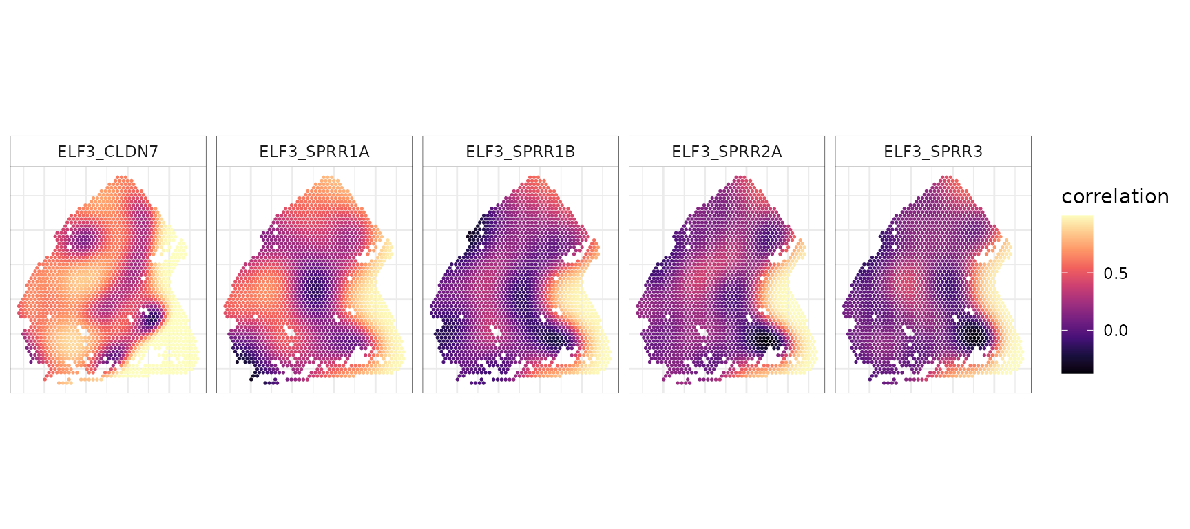

Identify gene pairs with significant SVC patterns

The spCorr also provides SVC testing to identify gene pairs whose correlations vary significantly across spatial locations. The BH-adjusted p-values from the SVC testing are stored in res$res_global.

pval_svc <- res$res_global
gene_pair_sig <- which(pval_svc < 0.05)
cat("Number of gene pairs with significant SVC patterns (FDR < 0.05):", length(gene_pair_sig), "\n")
#> Number of gene pairs with significant SVC patterns (FDR < 0.05): 294

Session information