Modeling spatially varying gene correlation along 1D spatial curve
Chenxin
(Flora) Jiang
Department of Statistics and Data Science, University
of California, Los Angeles
cflorajiang@g.ucla.edu
03 July 2026
Source:vignettes/spCorr-1D.Rmd
spCorr-1D.Rmd
library(spCorr)
library(Seurat)
library(purrr)
library(tibble)
library(ggplot2)
library(dplyr)
library(tidyr)
library(viridis)
library(MorphoGAM)
library(stats)
library(utils)
Introduction
This tutorial demonstrates how to use spCorr to (i) infer spot-level gene–gene correlations for specified gene pairs, and (ii) identify gene pairs exhibiting spatially varying correlation (SVC) patterns along a 1D spatial curve.
Prepare input data
In this example, we analyze a subset of the mouse brain cortex dataset generated using the 10x Xenium platform. The dataset is provided by 10x Genomics as part of the “Fresh Frozen Mouse Brain for Xenium Explorer Demo,” available at 10x Genomics.
## Load example ST data
# It contains a Seurat object
options(timeout = 3600)
tf <- tempfile(fileext = ".rds")
utils::download.file("https://ndownloader.figshare.com/files/66021356", tf, mode = "wb")
xenium.obj <- readRDS(tf)
unlink(tf)

xenium.obj <- UpdateSeuratObject(xenium.obj)
xenium.obj$ccf_region <- gsub("1|2/3|4|5|6a|6b", "", xenium.obj$ccf) %>%
  as.factor() %>%
  droplevels()

# Subset celltype L2/3 IT
celltype <- "L2/3 IT"
xenium_sub.obj <- xenium.obj[, xenium.obj$ensembled.celltype1 %in% celltype]
Now we prepare the input data for spCorr analysis.
# Count matrix
count_mat <- xenium_sub.obj[["Xenium"]]$counts
# Covariate matrix
cov_mat <- cbind(GetTissueCoordinates(xenium_sub.obj), xenium_sub.obj@meta.data)
rownames(cov_mat) <- colnames(count_mat)
Next we will use MorphoGAM (Nicol et al., 2024) to find the 1D spatial curve associated with the 2D spatial coordinates of the spots. The 1D curve will be used as a covariate in the spCorr analysis.
# Use MorphoGAM to find the 1D spatial curve
MorphoGAM_fit <- MorphoGAM::CurveFinder(cov_mat[, c("x", "y")] |> as.matrix(), knn = 5)
cov_mat$t <- MorphoGAM_fit$xyt$t

# (and plot)
df <- MorphoGAM_fit$xyt %>% arrange(t)
plot_curve <- ggplot(df, aes(x = x, y = y)) +
  geom_point(color = "gray70") +
  geom_path(aes(x = f1, y = f2, color = t)) +
  labs(title = paste(celltype, ": 1D spatial curve from MorphoGAM")) +
  scale_color_viridis_c(option = "magma") +
  coord_fixed() +
  scale_y_reverse() +
  theme_minimal()
plot_curve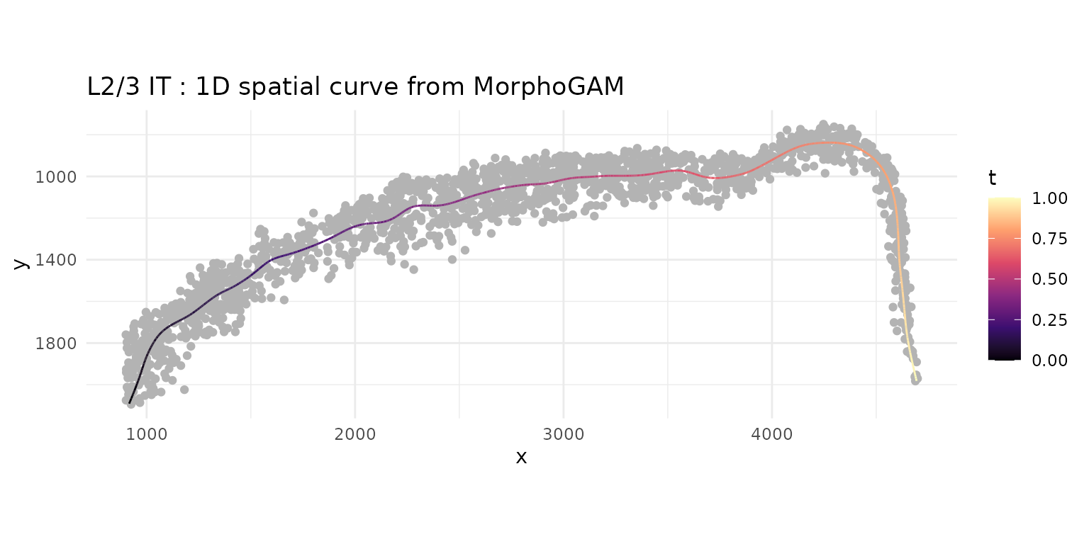
In this tutorial, we will focus on a subset of 10 genes that are highly expressed in the L2/3 IT cell type. We will analyze all possible gene pairs among these 10 genes.
Run spCorr
We now apply spCorr to infer spot-level gene–gene correlations for the selected gene pairs and to identify gene pairs with spatially varying correlation (SVC) pattern across the 1D spatial curve.
res <- spCorr(count_mat,
  gene_list,
  gene_pair_list,
  cov_mat,
  formula1 = "1",
  formula2 = "s(t, bs='tp', k=8)",
  return_pi = TRUE,
  ncores = 5,
  seed = 123
)
#> Start Marginal Fitting for 10 genes
#> Start Cross-Product Fitting for 45 gene pairs
Visualize spot-level correlations
We next visualize the inferred spot-level correlations and SVC patterns for specific gene pairs.
# Use the top gene pairs with the smallest FDR values for visualization
top_pairs <- names(sort(res$fdr))[1:6]

# Assemble spot-level correlation estimates and their confidence intervals
rho_df_long <- purrr::map_dfr(top_pairs, function(gp) {
  tibble::tibble(
    t = cov_mat$t, gene_pair = gp,
    rho = as.numeric(res$res_local[gp, ]),
    rho_lower = as.numeric(res$res_local_pi[[gp]]$lower),
    rho_upper = as.numeric(res$res_local_pi[[gp]]$upper)
  )
}) %>%
  dplyr::mutate(
    rho_lower = pmax(rho_lower, -1),
    rho_upper = pmin(rho_upper, 1),
    gene_pair = factor(gene_pair, levels = top_pairs)
  ) %>%
  dplyr::arrange(gene_pair, t)

# Visualize the estimated spot-level correlations along the 1D spatial curve
p_corr_t <- ggplot(rho_df_long, aes(x = t, y = rho)) +
  geom_ribbon(aes(ymin = rho_lower, ymax = rho_upper, group = gene_pair), fill = "purple", alpha = 0.25, color = NA) +
  geom_line(aes(group = gene_pair), color = "purple", linewidth = 0.6) +
  geom_hline(yintercept = 0, linetype = "dashed") +
  facet_wrap(~gene_pair, nrow = 2) +
  scale_x_continuous(breaks = c(0, 0.5, 1), labels = c("0", "0.5", "1")) +
  scale_y_continuous(breaks = c(-1, 0, 1), limits = c(-1, 1)) +
  labs(x = "t", y = "Correlation") +
  theme_minimal() +
  theme(
    aspect.ratio = 1 / 2,
    legend.position = "none",
    panel.grid = element_blank(),
    panel.border = element_rect(color = "black", fill = NA, linewidth = 0.2),
    strip.background = element_rect(color = "black", fill = NA, linewidth = 0.2),
    strip.text.x = element_text(face = "italic")
  )
p_corr_t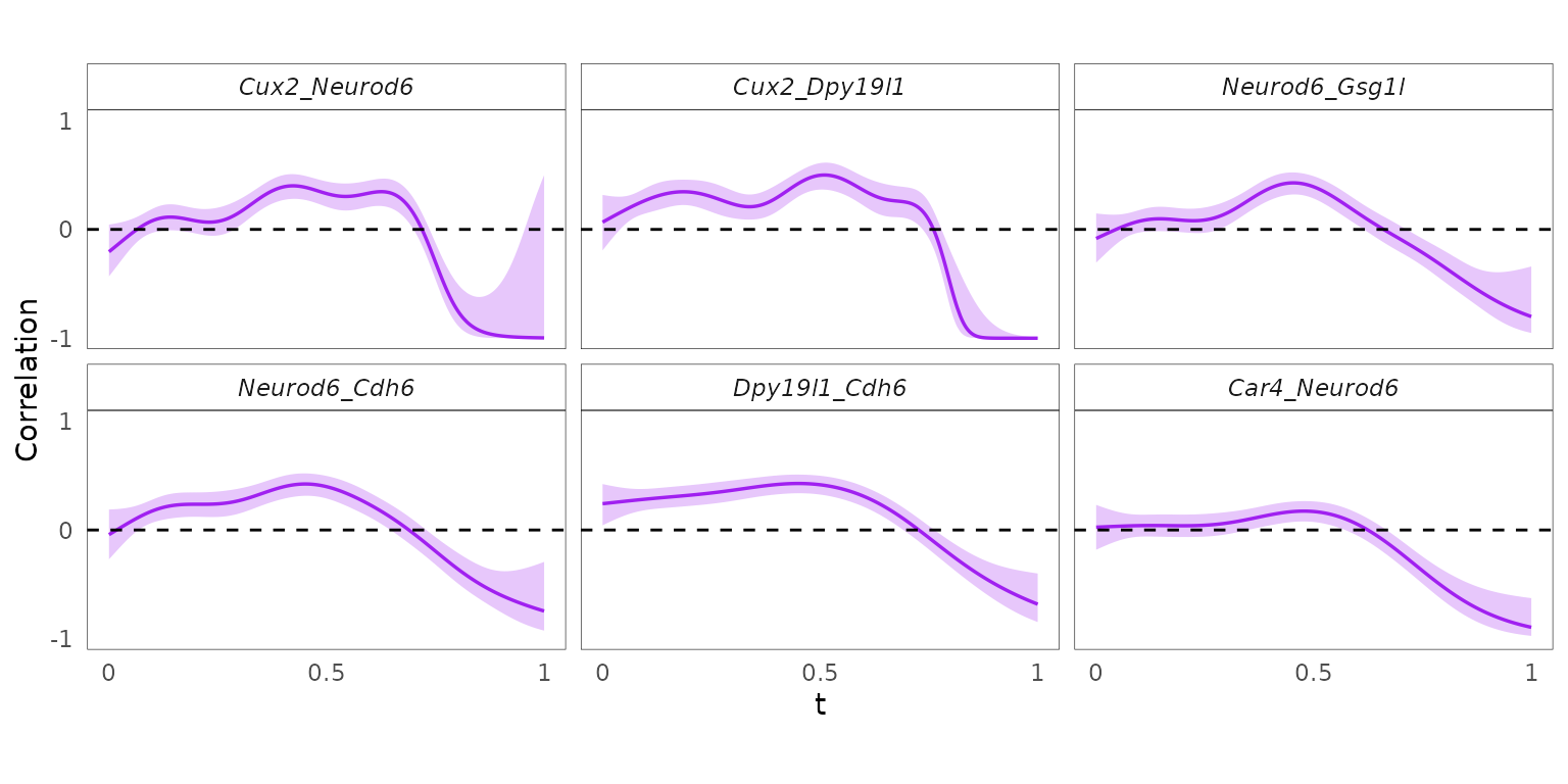
Session information
sessionInfo()
#> R version 4.2.3 (2023-03-15)
#> Platform: x86_64-pc-linux-gnu (64-bit)
#> Running under: Ubuntu 22.04.5 LTS
#>
#> Matrix products: default
#> BLAS:   /usr/lib/x86_64-linux-gnu/openblas-pthread/libblas.so.3
#> LAPACK: /usr/lib/x86_64-linux-gnu/openblas-pthread/libopenblasp-r0.3.20.so
#>
#> locale:
#>  [1] LC_CTYPE=en_US.UTF-8       LC_NUMERIC=C
#>  [3] LC_TIME=en_US.UTF-8        LC_COLLATE=en_US.UTF-8
#>  [5] LC_MONETARY=en_US.UTF-8    LC_MESSAGES=en_US.UTF-8
#>  [7] LC_PAPER=en_US.UTF-8       LC_NAME=C
#>  [9] LC_ADDRESS=C               LC_TELEPHONE=C
#> [11] LC_MEASUREMENT=en_US.UTF-8 LC_IDENTIFICATION=C
#>
#> attached base packages:
#> [1] stats     graphics  grDevices utils     datasets  methods   base
#>
#> other attached packages:
#>  [1] MorphoGAM_1.0.0    viridis_0.6.5      viridisLite_0.4.2  tidyr_1.3.2
#>  [5] dplyr_1.1.4        ggplot2_4.0.1      tibble_3.3.1       purrr_1.2.1
#>  [9] Seurat_5.4.0       SeuratObject_5.3.0 sp_2.2-0           spCorr_1.0.0.0000
#> [13] BiocStyle_2.26.0
#>
#> loaded via a namespace (and not attached):
#>   [1] spatstat.univar_3.1-6  spam_2.11-3            systemfonts_1.3.1
#>   [4] plyr_1.8.9             igraph_2.2.1           lazyeval_0.2.2
#>   [7] nanonext_1.7.2         splines_4.2.3          RcppHNSW_0.6.0
#>  [10] listenv_0.10.0         scattermore_1.2        digest_0.6.39
#>  [13] gratia_0.11.1          invgamma_1.2           htmltools_0.5.9
#>  [16] SQUAREM_2021.1         magrittr_2.0.4         tensor_1.5.1
#>  [19] cluster_2.1.6          ROCR_1.0-12            globals_0.19.1
#>  [22] dimRed_0.2.7           matrixStats_1.5.0      pkgdown_2.2.0
#>  [25] spatstat.sparse_3.1-0  princurve_2.1.6        ggrepel_0.9.6
#>  [28] textshaping_1.0.4      xfun_0.56              jsonlite_2.0.0
#>  [31] progressr_0.18.0       spatstat.data_3.1-9    survival_3.7-0
#>  [34] zoo_1.8-15             ape_5.8-1              glue_1.8.1
#>  [37] DRR_0.0.4              polyclip_1.10-7        gtable_0.3.6
#>  [40] kernlab_0.9-33         future.apply_1.20.1    abind_1.4-8
#>  [43] scales_1.4.0           spatstat.random_3.4-4  miniUI_0.1.2
#>  [46] Rcpp_1.1.1             xtable_1.8-4           reticulate_1.44.1
#>  [49] dotCall64_1.2          tweedie_2.3.5          truncnorm_1.0-9
#>  [52] htmlwidgets_1.6.4      httr_1.4.7             RColorBrewer_1.1-3
#>  [55] ica_1.0-3              pkgconfig_2.0.3        farver_2.1.2
#>  [58] sass_0.4.10            uwot_0.2.4             deldir_2.0-4
#>  [61] labeling_0.4.3         tidyselect_1.2.1       rlang_1.1.7
#>  [64] reshape2_1.4.5         later_1.4.5            tools_4.2.3
#>  [67] cachem_1.1.0           mirai_2.5.3            cli_3.6.6
#>  [70] generics_0.1.4         ggridges_0.5.7         evaluate_1.0.5
#>  [73] stringr_1.6.0          fastmap_1.2.0          yaml_2.3.12
#>  [76] ragg_1.5.0             goftest_1.2-3          knitr_1.51
#>  [79] fs_2.1.0               fitdistrplus_1.2-6     RANN_2.6.2
#>  [82] pbapply_1.7-4          future_1.69.0          nlme_3.1-164
#>  [85] mime_0.13              mvnfast_0.2.8          compiler_4.2.3
#>  [88] rstudioapi_0.18.0      ggokabeito_0.1.0       plotly_4.12.0
#>  [91] png_0.1-8              spatstat.utils_3.2-1   bslib_0.10.0
#>  [94] stringi_1.8.7          desc_1.4.3             RSpectra_0.16-2
#>  [97] lattice_0.22-6         Matrix_1.6-5           vctrs_0.7.1
#> [100] pillar_1.11.1          lifecycle_1.0.5        BiocManager_1.30.27
#> [103] spatstat.geom_3.7-0    lmtest_0.9-40          jquerylib_0.1.4
#> [106] RcppAnnoy_0.0.23       data.table_1.18.4      cowplot_1.2.0
#> [109] irlba_2.3.7            httpuv_1.6.16          patchwork_1.3.2
#> [112] R6_2.6.1               bookdown_0.46          promises_1.5.0
#> [115] KernSmooth_2.23-24     gridExtra_2.3          parallelly_1.46.1
#> [118] codetools_0.2-20       dichromat_2.0-0.1      gtools_3.9.5
#> [121] fastDummies_1.7.5      MASS_7.3-58.2          CVST_0.2-3
#> [124] withr_3.0.2            sctransform_0.4.3      mgcv_1.9-3
#> [127] parallel_4.2.3         grid_4.2.3             rmarkdown_2.30
#> [130] ashr_2.2-63            S7_0.2.1               otel_0.2.0
#> [133] Rtsne_0.17             mixsqp_0.3-54          spatstat.explore_3.7-0
#> [136] shiny_1.12.1