Modeling varying gene correlation across spatial domains and cell types
Chenxin
(Flora) Jiang
Department of Statistics and Data Science, University
of California, Los Angeles
cflorajiang@g.ucla.edu
03 July 2026
Source:vignettes/spCorr-sc.Rmd
spCorr-sc.Rmd
library(spCorr)
library(Seurat)
library(purrr)
library(tibble)
library(ggplot2)
library(dplyr)
library(tidyr)
library(viridis)
library(MorphoGAM)
library(stats)
library(utils)
Introduction
This tutorial demonstrates how to use spCorr to model varying gene-gene correlations in two settings:
spatial transcriptomics data, where correlations may vary across spatial domains; and
single-cell RNA-seq data, where correlations may vary across cell types.
We illustrate the workflow using mouse brain hippocampal CA1, CA2, and CA3 populations from Visium HD spatial transcriptomics data and matched scRNA-seq reference data.
Visium HD data
In this example, we analyze a subset of the mouse brain hippocampus dataset generated using the 10x Visium HD platform. The dataset is provided by 10x Genomics as part of the “Visium HD Spatial Gene Expression Library, Mouse Brain (FFPE),” available at 10x Genomics. We focus on spatially distinct hippocampal structures corresponding to the pyramidal layer and annotate this region into CA1, CA2, and CA3 domains based on canonical marker genes.
## Load example ST data
# counts_hippo, cov_mat_hippo
tf1 <- tempfile(fileext = ".RData")
utils::download.file("https://ndownloader.figshare.com/files/66271418", tf1, mode = "wb")
load(tf1)
unlink(tf1)
The downloaded data contain a spot-level count matrix
(counts_hippo) and a corresponding covariate matrix
(cov_mat_hippo) that includes spot coordinates and spatial
domain annotations.
Visualize the spatial domain annotation of the Visium HD data. The
domain labels are stored in the annotation column of
cov_mat_hippo.
custom_colors <- c("CA1" = "#66c2a5",
                   "CA2" = "#fc8d62",
                   "CA3" = "#8da0cb")

p_domain <-  ggplot(cov_mat_hippo, aes(x = x2, y = -x1, color = annotation)) +
  ggrastr::geom_point_rast(size = 0.3, na.rm = TRUE) +
  scale_color_manual(values = custom_colors,
                     guide = guide_legend(override.aes = list(size = 2))) +
  labs(x = NULL, y = NULL, color = NULL) +
  theme_minimal() +
  coord_fixed() +
  theme(legend.position = "bottom",
        axis.ticks = element_blank(),
        panel.grid = element_blank(),
        axis.text = element_blank(),
        panel.border = element_rect(color = "black", fill = NA, linewidth = 0.2)) +
  ggtitle("Spatial domain annotation of the Visium HD data")

p_domain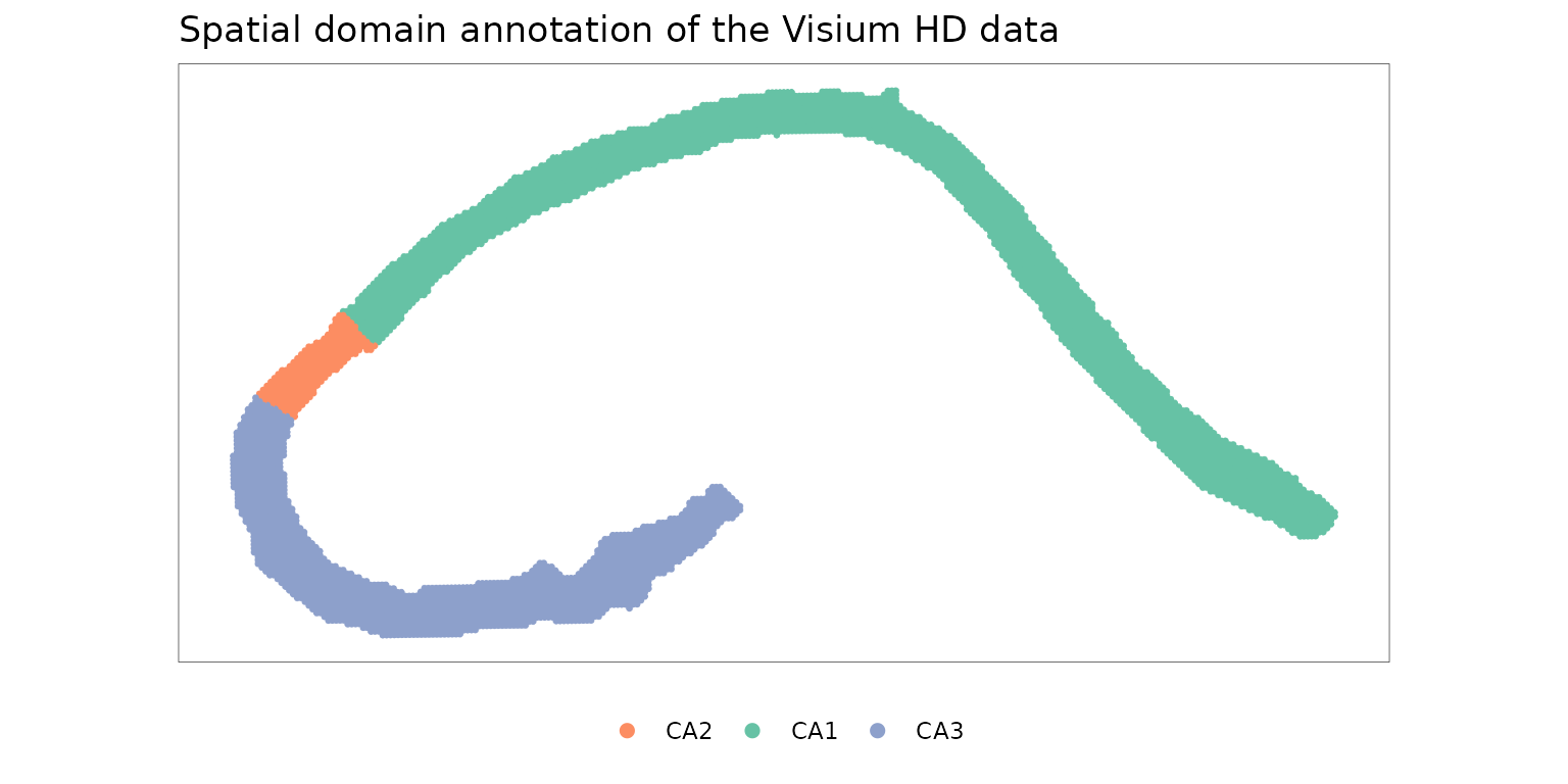
To illustrate the workflow, we next focus on a small set of genes that are highly expressed in the CA1, CA2, and CA3 hippocampal domains. We consider all possible gene pairs among these genes for downstream correlation analysis.
gene_list <- c("Camk2a", "Slc1a2", "Ptk2b", "Nrgn", "Snap25")
gene_pair_list <- t(combn(gene_list, 2))
rownames(gene_pair_list) <- apply(gene_pair_list, 1, paste0, collapse = "_")
Run spCorr
We apply spCorr to infer spot-level gene–gene correlations and identify gene pairs with spatially varying correlation patterns across hippocampal domains.
res <- spCorr(counts_hippo,
  gene_list,
  gene_pair_list,
  cov_mat_hippo,
  formula1 = "1",
  formula2 = "annotation",
  ncores = 5,
  seed = 123
)
#> Start Marginal Fitting for 5 genes
#> Start Cross-Product Fitting for 10 gene pairs
Visualize spot-level correlations
We next visualize the inferred spot-level correlations and SVC patterns for specific gene pairs.
# Use the top gene pairs with the smallest FDR values for visualization
top_pairs <- names(sort(res$fdr))[1:6]

# Assemble spot-level correlation estimates and their confidence intervals
rho_df_long <- purrr::map_dfr(top_pairs, function(gp) {
  tibble::tibble(
    x = cov_mat_hippo$x2, y = cov_mat_hippo$x1, gene_pair = gp,
    rho = as.numeric(res$res_local[gp, ])
  )
}) %>%
  dplyr::mutate(gene_pair = factor(gene_pair, levels = top_pairs))

# Visualize the estimated spot-level correlations across 2D space
p_corr_d <- ggplot(rho_df_long, aes(x = x, y = y, color = rho)) +
  geom_point(size = 0.3) +
  facet_wrap(~gene_pair, nrow = 2) +
  coord_fixed() +
  scale_y_reverse() +
  scale_color_gradient2(low = "blue", mid = "white", high = "red", midpoint = 0, limits = c(-1, 1), name = "Correlation") +
  theme_minimal() +
  theme(
    legend.position = "right",
    axis.title = element_blank(),
    axis.text = element_blank(),
    axis.ticks = element_blank(),
    panel.grid = element_blank(),
    panel.border = element_rect(color = "black", fill = NA, linewidth = 0.2),
    strip.background = element_rect(color = "black", fill = NA, linewidth = 0.2),
    strip.text.x = element_text(face = "italic")
  )

p_corr_d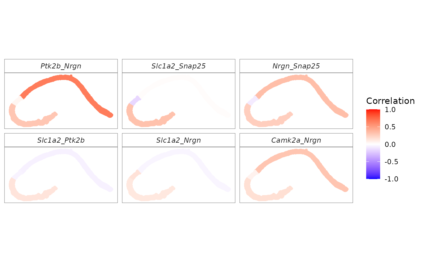
scRNA-seq data
As a comparison, we analyze scRNA-seq reference data containing CA1, CA2, and CA3 principal cells. The single-cell RNA-seq hippocampus dataset is available as a processed Seurat object from Dropbox, with raw count matrices downloadable from the DropViz website.
Unlike the spatial transcriptomics example, here the grouping variable is the annotated cell type. Consequently, spCorr is used to identify gene pairs whose correlations vary across cell types rather than across spatial domains.
## Load reference scRNA-seq data
# counts_hippo, cov_mat_hippo
options(timeout = 3600)
tf2 <- tempfile(fileext = ".rds")
utils::download.file("https://ndownloader.figshare.com/files/66276401", tf2, mode = "wb")
obj_sc <- readRDS(tf2)
unlink(tf2)
We first extract the normalized expression matrix, cell metadata, and UMAP coordinates from the Seurat object. The UMAP coordinates are included in the covariate matrix for visualization purposes only and are not used when fitting the model.
# Count matrix
counts_hippo_sc <- GetAssayData(obj_sc, layer='data')
# Covariate matrix
cov_hippo_sc <- obj_sc@meta.data
rownames(cov_hippo_sc) <- colnames(counts_hippo_sc)
cov_hippo_sc$celltype <- factor(cov_hippo_sc$celltype,
                                levels = c("CA2 Principal cells",
                                           "CA1 Principal cells",
                                           "CA3 Principal cells"))
umap_df <- Embeddings(obj_sc, "umap") %>% as.data.frame()
cov_hippo_sc <- cbind(cov_hippo_sc, umap_df)
The UMAP embedding illustrates the annotated CA1, CA2, and CA3 principal cell populations used in the downstream analysis.
custom_colors <- c(
  "CA1 Principal cells" = "#66c2a5",
  "CA2 Principal cells" = "#fc8d62",
  "CA3 Principal cells" = "#8da0cb")

p_umap <- DimPlot(obj_sc, reduction = "umap",
                  group.by = "celltype",
                  cols = custom_colors,
                  label = TRUE, repel = TRUE) +
  ggtitle("Cell type annotation of the scRNA-seq data")

p_umap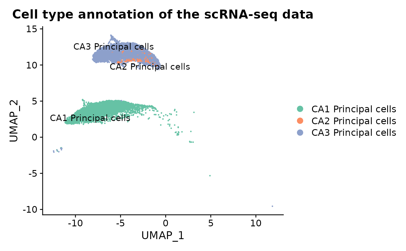
Run spCorr
Using the same set of genes as in the Visium HD example (converted to uppercase to match the scRNA-seq gene symbols), we apply spCorr to estimate cell-level gene–gene correlations and identify gene pairs whose correlations vary across cell types.
gene_List <- toupper(gene_list)
gene_pair_List = t(combn(gene_List, 2))
rownames(gene_pair_List) <- apply(gene_pair_List, 1, paste0, collapse = "_")

res_sc <- spCorr(counts_hippo_sc,
  gene_List,
  gene_pair_List,
  cov_hippo_sc,
  formula1 = "1",
  formula2 = "celltype",
  ncores = 5,
  seed = 123
)
#> Start Marginal Fitting for 5 genes
#> Start Cross-Product Fitting for 10 gene pairs
Visualize cell-level correlations
We next visualize the estimated cell-level correlations for the most significant gene pairs on the UMAP embedding.
# Use the top gene pairs with the smallest FDR values for visualization
top_pairs <- names(sort(res_sc$fdr))[1:6]

# Assemble spot-level correlation estimates and their confidence intervals
rho_df_long <- purrr::map_dfr(top_pairs, function(gp) {
  tibble::tibble(
    x = cov_hippo_sc$UMAP_1, y = cov_hippo_sc$UMAP_2, gene_pair = gp,
    rho = as.numeric(res_sc$res_local[gp, ])
  )
}) %>%
  dplyr::mutate(gene_pair = factor(gene_pair, levels = top_pairs))

# Visualize the estimated spot-level correlations across 2D space
p_corr_sc <- ggplot(rho_df_long, aes(x = x, y = -y, color = rho)) +
  geom_point(size = 0.3) +
  facet_wrap(~gene_pair, nrow = 2) +
  coord_fixed() +
  scale_y_reverse() +
  scale_color_gradient2(low = "blue", mid = "white", high = "red", midpoint = 0, limits = c(-1, 1), name = "Correlation") +
  theme_minimal() +
  theme(
    legend.position = "right",
    axis.title = element_blank(),
    axis.text = element_blank(),
    axis.ticks = element_blank(),
    panel.grid = element_blank(),
    panel.border = element_rect(color = "black", fill = NA, linewidth = 0.2),
    strip.background = element_rect(color = "black", fill = NA, linewidth = 0.2),
    strip.text.x = element_text(face = "italic")
  )

p_corr_sc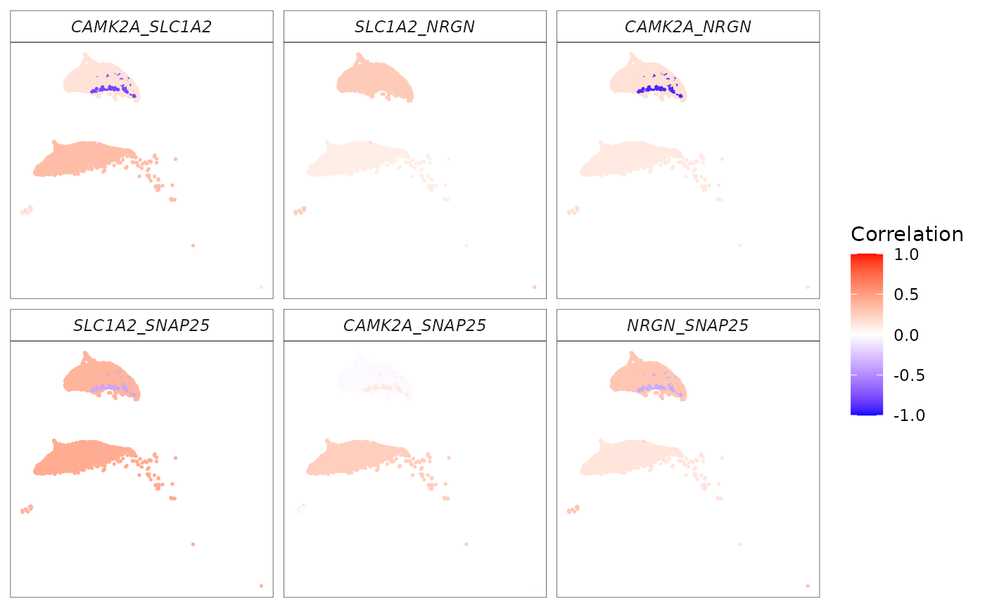
Session information
sessionInfo()
#> R version 4.2.3 (2023-03-15)
#> Platform: x86_64-pc-linux-gnu (64-bit)
#> Running under: Ubuntu 22.04.5 LTS
#>
#> Matrix products: default
#> BLAS:   /usr/lib/x86_64-linux-gnu/openblas-pthread/libblas.so.3
#> LAPACK: /usr/lib/x86_64-linux-gnu/openblas-pthread/libopenblasp-r0.3.20.so
#>
#> locale:
#>  [1] LC_CTYPE=en_US.UTF-8       LC_NUMERIC=C
#>  [3] LC_TIME=en_US.UTF-8        LC_COLLATE=en_US.UTF-8
#>  [5] LC_MONETARY=en_US.UTF-8    LC_MESSAGES=en_US.UTF-8
#>  [7] LC_PAPER=en_US.UTF-8       LC_NAME=C
#>  [9] LC_ADDRESS=C               LC_TELEPHONE=C
#> [11] LC_MEASUREMENT=en_US.UTF-8 LC_IDENTIFICATION=C
#>
#> attached base packages:
#> [1] stats     graphics  grDevices utils     datasets  methods   base
#>
#> other attached packages:
#>  [1] MorphoGAM_1.0.0    viridis_0.6.5      viridisLite_0.4.2  tidyr_1.3.2
#>  [5] dplyr_1.1.4        ggplot2_4.0.1      tibble_3.3.1       purrr_1.2.1
#>  [9] Seurat_5.4.0       SeuratObject_5.3.0 sp_2.2-0           spCorr_1.0.0.0000
#> [13] BiocStyle_2.26.0
#>
#> loaded via a namespace (and not attached):
#>   [1] spatstat.univar_3.1-6  spam_2.11-3            systemfonts_1.3.1
#>   [4] plyr_1.8.9             igraph_2.2.1           lazyeval_0.2.2
#>   [7] nanonext_1.7.2         splines_4.2.3          RcppHNSW_0.6.0
#>  [10] listenv_0.10.0         scattermore_1.2        digest_0.6.39
#>  [13] gratia_0.11.1          invgamma_1.2           htmltools_0.5.9
#>  [16] SQUAREM_2021.1         magrittr_2.0.4         tensor_1.5.1
#>  [19] cluster_2.1.6          ROCR_1.0-12            globals_0.19.1
#>  [22] dimRed_0.2.7           matrixStats_1.5.0      pkgdown_2.2.0
#>  [25] spatstat.sparse_3.1-0  princurve_2.1.6        ggrepel_0.9.6
#>  [28] textshaping_1.0.4      xfun_0.56              jsonlite_2.0.0
#>  [31] progressr_0.18.0       spatstat.data_3.1-9    survival_3.7-0
#>  [34] zoo_1.8-15             ape_5.8-1              glue_1.8.1
#>  [37] DRR_0.0.4              polyclip_1.10-7        gtable_0.3.6
#>  [40] kernlab_0.9-33         future.apply_1.20.1    abind_1.4-8
#>  [43] scales_1.4.0           spatstat.random_3.4-4  miniUI_0.1.2
#>  [46] Rcpp_1.1.1             xtable_1.8-4           reticulate_1.44.1
#>  [49] dotCall64_1.2          tweedie_2.3.5          truncnorm_1.0-9
#>  [52] htmlwidgets_1.6.4      httr_1.4.7             RColorBrewer_1.1-3
#>  [55] ica_1.0-3              pkgconfig_2.0.3        farver_2.1.2
#>  [58] sass_0.4.10            uwot_0.2.4             deldir_2.0-4
#>  [61] labeling_0.4.3         tidyselect_1.2.1       rlang_1.1.7
#>  [64] reshape2_1.4.5         later_1.4.5            tools_4.2.3
#>  [67] cachem_1.1.0           mirai_2.5.3            cli_3.6.6
#>  [70] generics_0.1.4         ggridges_0.5.7         evaluate_1.0.5
#>  [73] stringr_1.6.0          fastmap_1.2.0          yaml_2.3.12
#>  [76] ragg_1.5.0             goftest_1.2-3          knitr_1.51
#>  [79] fs_2.1.0               fitdistrplus_1.2-6     RANN_2.6.2
#>  [82] pbapply_1.7-4          future_1.69.0          nlme_3.1-164
#>  [85] mime_0.13              ggrastr_1.0.2          mvnfast_0.2.8
#>  [88] compiler_4.2.3         rstudioapi_0.18.0      beeswarm_0.4.0
#>  [91] ggokabeito_0.1.0       plotly_4.12.0          png_0.1-8
#>  [94] spatstat.utils_3.2-1   bslib_0.10.0           stringi_1.8.7
#>  [97] desc_1.4.3             RSpectra_0.16-2        lattice_0.22-6
#> [100] Matrix_1.6-5           vctrs_0.7.1            pillar_1.11.1
#> [103] lifecycle_1.0.5        BiocManager_1.30.27    spatstat.geom_3.7-0
#> [106] lmtest_0.9-40          jquerylib_0.1.4        RcppAnnoy_0.0.23
#> [109] data.table_1.18.4      cowplot_1.2.0          irlba_2.3.7
#> [112] httpuv_1.6.16          patchwork_1.3.2        R6_2.6.1
#> [115] bookdown_0.46          promises_1.5.0         KernSmooth_2.23-24
#> [118] gridExtra_2.3          vipor_0.4.7            parallelly_1.46.1
#> [121] codetools_0.2-20       dichromat_2.0-0.1      gtools_3.9.5
#> [124] fastDummies_1.7.5      MASS_7.3-58.2          CVST_0.2-3
#> [127] withr_3.0.2            sctransform_0.4.3      mgcv_1.9-3
#> [130] parallel_4.2.3         grid_4.2.3             rmarkdown_2.30
#> [133] ashr_2.2-63            S7_0.2.1               otel_0.2.0
#> [136] Cairo_1.7-0            Rtsne_0.17             mixsqp_0.3-54
#> [139] spatstat.explore_3.7-0 shiny_1.12.1           ggbeeswarm_0.7.3